🧩 Extra: Node-by-node phenological mapping
Node-by-node phenological mapping is the plant-by-plant record of what is at each position of each reproductive node of the cotton plant: square, flower, boll, open boll or aborted structure. In upCampo it has three parts: collection in the app, done by the scout in the field; the phenology dashboard, which draws the plant node by node from that collection; and the reports, especially MON.02.01 (formerly 001.N) - Summary Phenology and MON.02.05 (formerly 001.M) - Detailed Phenology.
What this map answers is where the plant is holding its load and where it is losing it: at which nodes the bolls set, at what height on the plant abortion is concentrated, how much has already opened. That is information the count of squares and bolls per meter doesn't give, because it says how much there is, but not where.
- The scout measures the plant in the app, within the scouting: height, vegetative nodes and, node by node, what is at each position on the branch.
- The phone syncs and, within a few minutes, upCampo turns each plant into a drawing of the plant.
- The agronomist reads the plant on the dashboard, in the field summary or plant by plant, and compares dates or fields side by side.
- The reports bring the same data in numbers and on paper: MON.02.01 (formerly 001.N) with the field's percentages and averages, MON.02.02 (formerly 001.M2) with each plant's drawing.
📍 Where each part is
| Part | Where |
|---|---|
| Collection | App, Scouting (IPM) menu → field → New Scouting → Detailed Cotton Phenology class |
| Dashboard | The Phenology page, opened at the dedicated address upCampo gives the farm — it is not in the web portal menu |
| Reports | Web portal, Reports menu, Survey theme: MON.02.01 (formerly 001.N) - Summary Phenology and MON.02.05 (formerly 001.M) - Detailed Phenology |
1. Collection in the app
App: Scouting (IPM) > New Scouting > Detailed Cotton Phenology
The measurement happens within a regular scouting. After opening the point, the scout selects the Detailed Cotton Phenology class in the pest list, chooses the plant (Plant 1, Plant 2…) and fills in its screen:
- Height, Veg. Node Qty (vegetative nodes) and Veg. Square Qty (vegetative squares).
- One tap on + for each reproductive node. The grid gets one row per node, numbered from the last vegetative node — with 6 vegetative nodes, the first reproductive one is Node 7. The Total Node Qty is calculated automatically.
- On each node, positions 1 to 5 on the branch, from closest to the stem to farthest. Each tap advances one state: Abs. (absent) → Square → Flower → Boll → Open (open boll) → Abor. (aborted).
- SAVE.
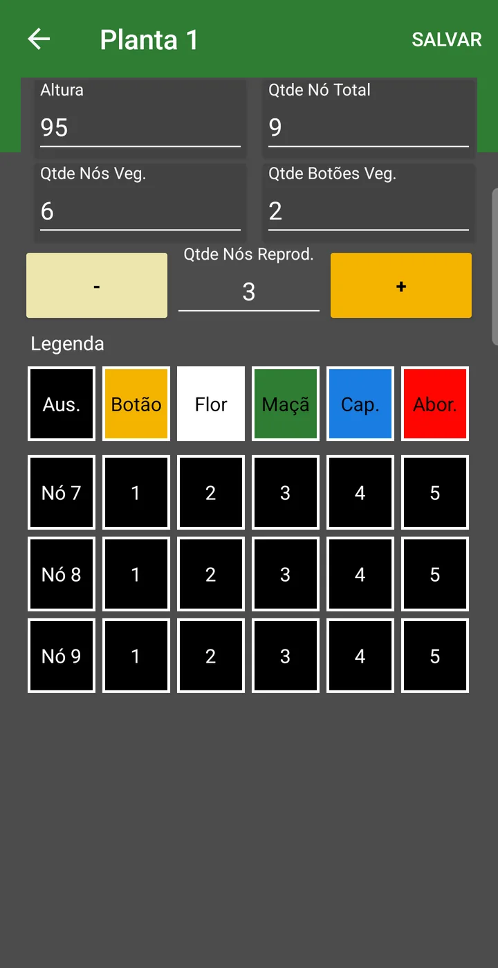
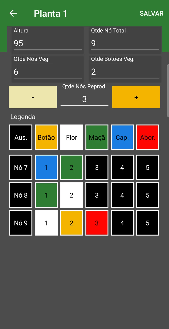
The complete step by step for the plant screen, with all the screenshots, is in the Quick Guide - Pest Monitoring.
Absent positions are not saved. The app saves one record for each measurement and one for each position marked with a state; whatever was left as Abs. does not become a record. This matters when reading the percentages, further below.
Counting structures per meter
A second measurement goes into the same scouting; it is not by node and feeds the MON.02.03 (formerly 001.O) report: the Structure per meter pest. It appears in the point's pest list, inside the class of the same name, and instead of a grid it opens four fields to type in:
| Field | What to enter |
|---|---|
| Meters assessed | The stretch of row walked at that point. How much to measure is up to the farm — in the cotton scouting for the 2026 season, most use 5 meters per point. |
| Total plants | How many plants there are in that stretch. This is where the report's stand per meter comes from. |
| Total structures | How many structures were counted in the stretch. |
| Average weight | The average weight of the structure, in grams. It goes straight into the arroba estimate; in the 2026 season the values entered range between 4 and 5.5 g. |
The report adds up the field's points: with 6 points of 3 meters, for example, it shows 18 meters assessed and the total plants and structures from all of them. This count produces the stand, the average per meter and the estimated @ in MON.02.03 (formerly 001.O).
2. The phenology dashboard
Phenology page (the farm's dedicated address)
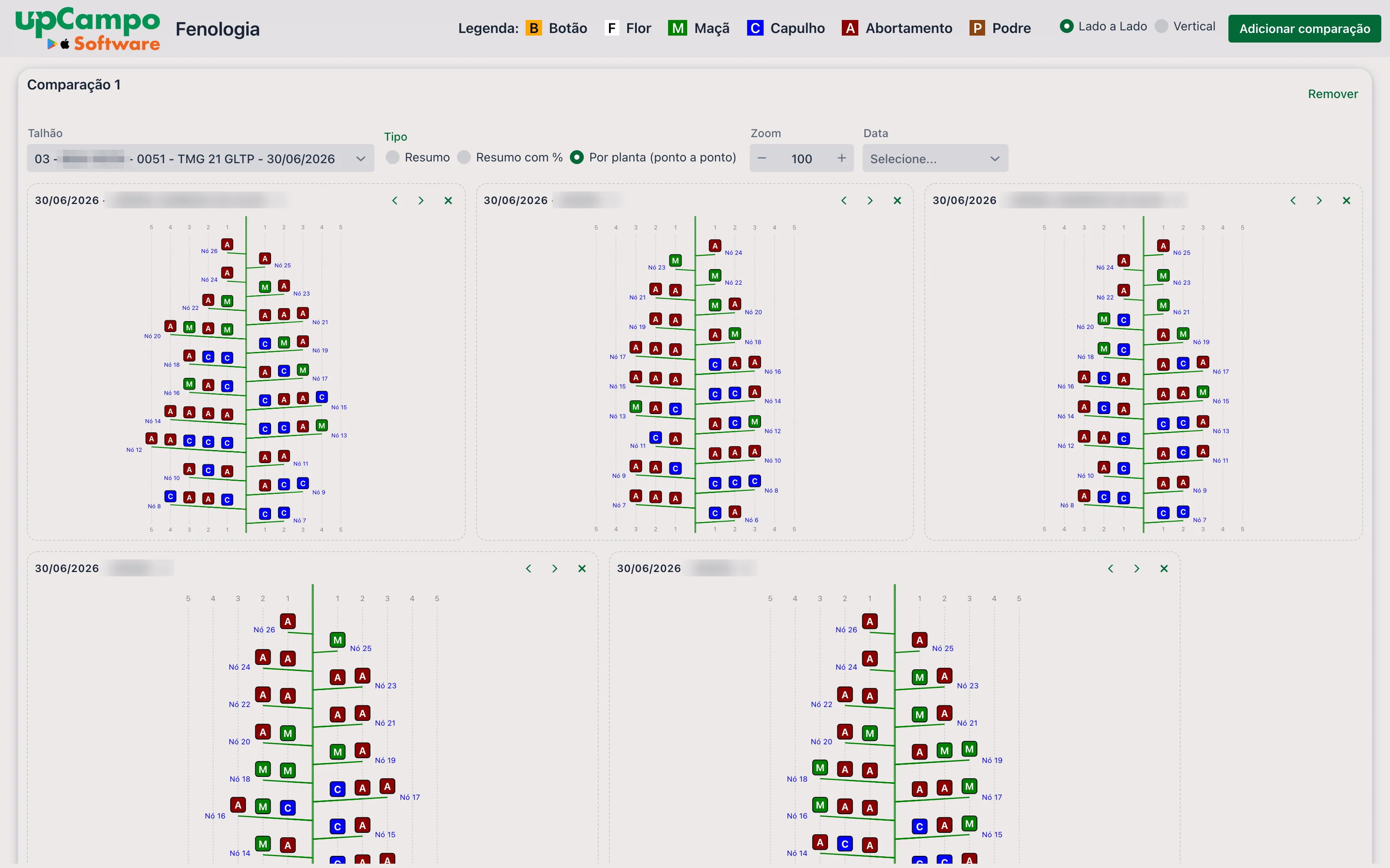
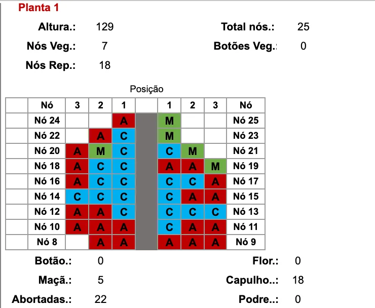
The dashboard shows the cotton plant as it is in the field: the stem in the center, the reproductive nodes rising and alternating sides, and on each branch positions 1 to 5 with the letter and color of what was found. It opens with the header and an empty comparison area.
In the header:
| Item | What it does |
|---|---|
| Legend | B Square (orange), F Flower (white), M Boll (green), C Open boll (blue), A Abortion (dark red) and P Rotten (brown). The app doesn't have the Rotten state in the plant grid, so it doesn't show up in collections made there. |
| Side by Side / Vertical | How comparisons are arranged: all in the same strip, one next to the other, or one below the other. |
| Add comparison | Opens another comparison area (Comparison 2, 3…), each with its own filters. |
In each comparison:
| Field | Description |
|---|---|
| Field | The field, variety and scouting date, on a single line — for example, 03 - … - TMG 21 GLTP - 30/06/2026. Each measured date is one item: the same field appears once per collection day. |
| Type | Summary, Summary with % or Per plant (point by point) — explained below. |
| Zoom | Size of the drawings, from 50 to 200. Increase it to read the percentages. |
| Date | Filters the Field list to show only scouting from that day. Left empty, the list shows all dates. |
| Remove | Takes the comparison off the screen. |
Each drawing has, in the corner, the ‹ and › arrows, which change the order of the drawings, and the ✕, which removes that drawing from the screen. None of this changes data: the dashboard is view-only, and whatever you rearrange goes back to normal when the page is reloaded.
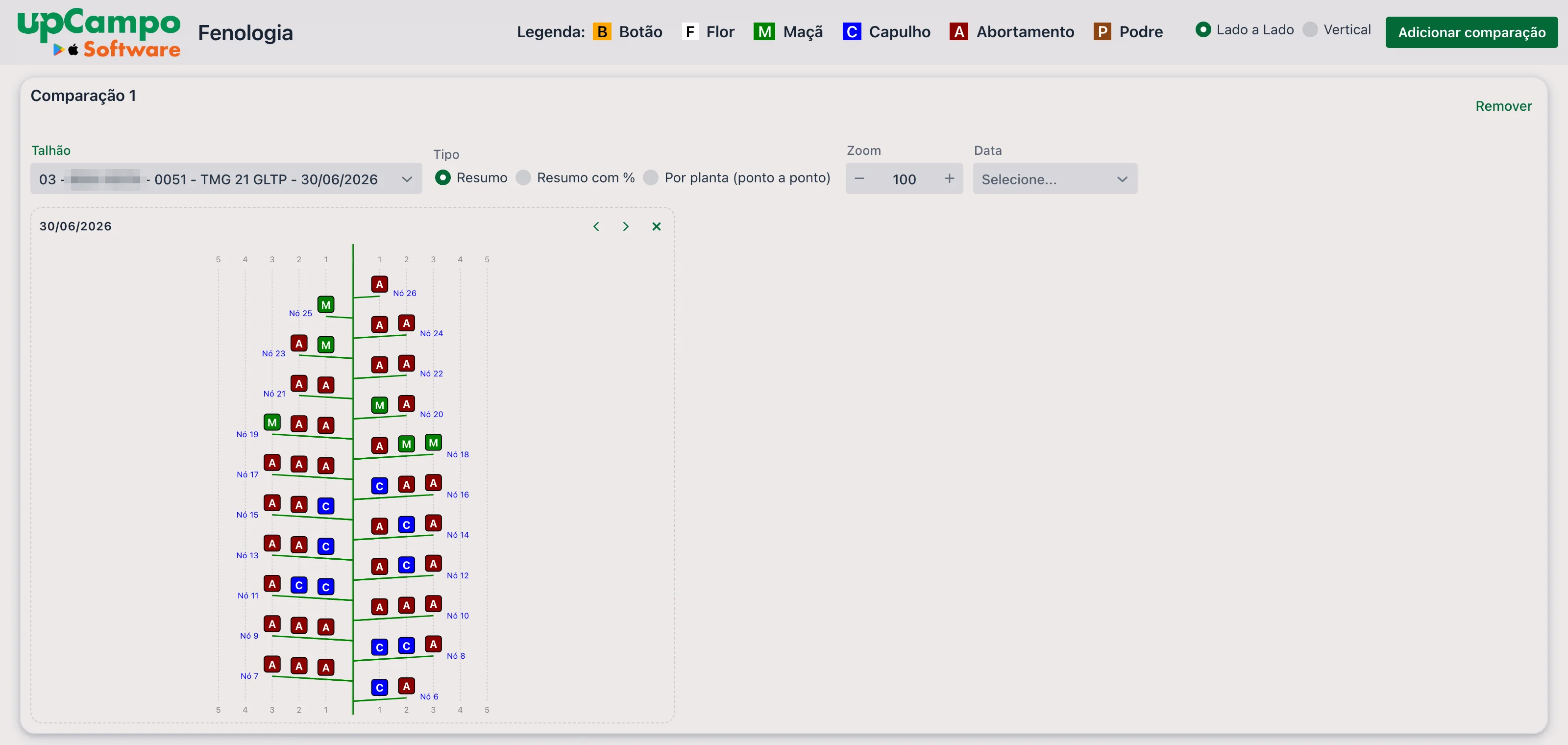
Summary
A single plant drawing, representing the field on that day. At each node and position, the most frequent state among the plants measured appears. It is the quick read: where the load is, where the abortion is.
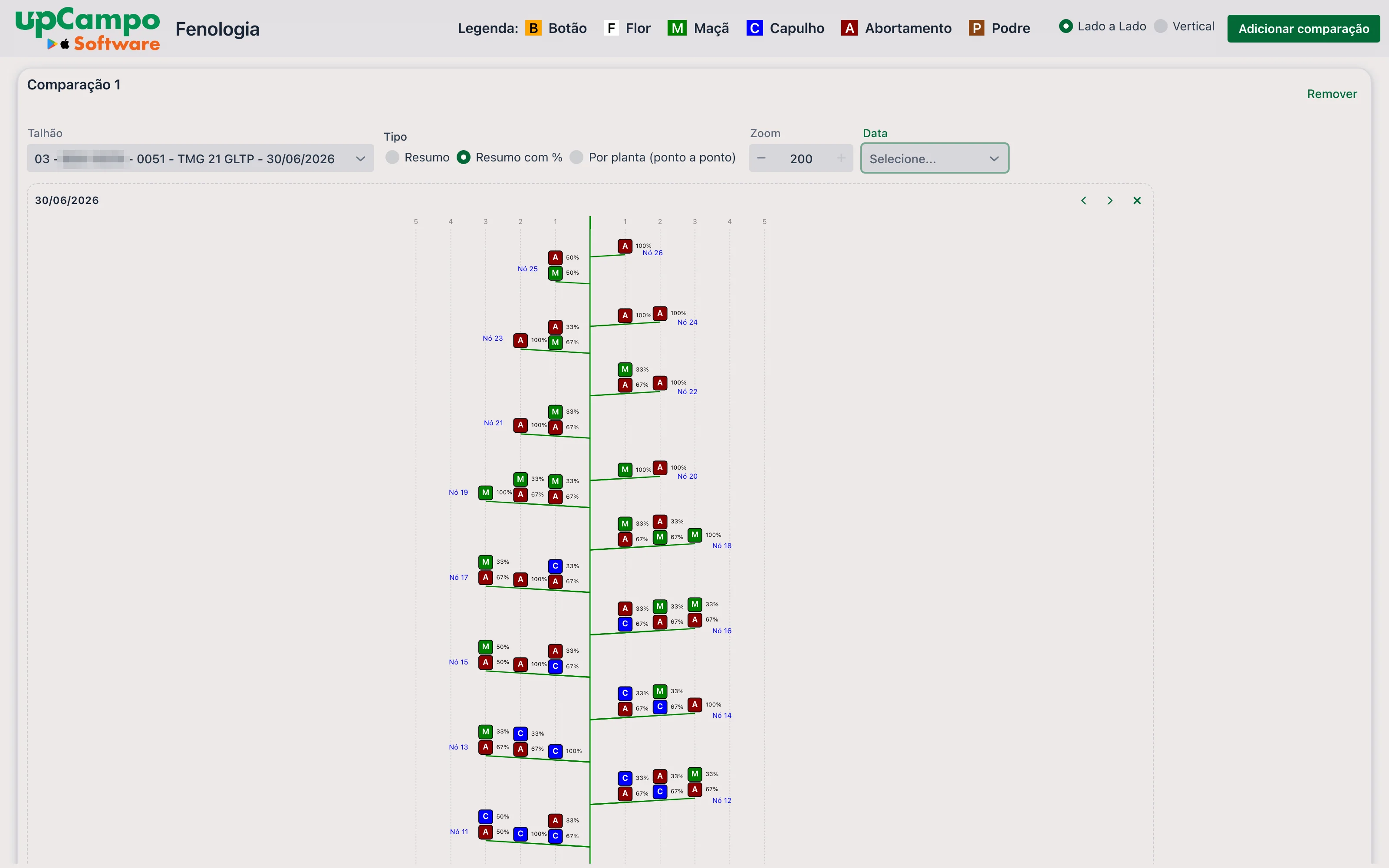
Summary with %
The same drawing, but at each position all the states found appear, stacked, each with its percentage. In the example below, position 1 on Node 25 shows A 50% and M 50%: half the plants had an aborted structure there, half a boll.
Per plant (point by point)
One drawing for each scouting point — that is, for each plant measured. The title of each drawing shows the date, the scout who measured and the point number. This is where you check the variation between plants and find a measurement that is out of line.
Comparing dates or fields
With Add comparison, the screen gets a second area with its own filters. The most common use is the same field on two dates, to see the plant develop; it also works for putting two fields, or two varieties, side by side on the same date.
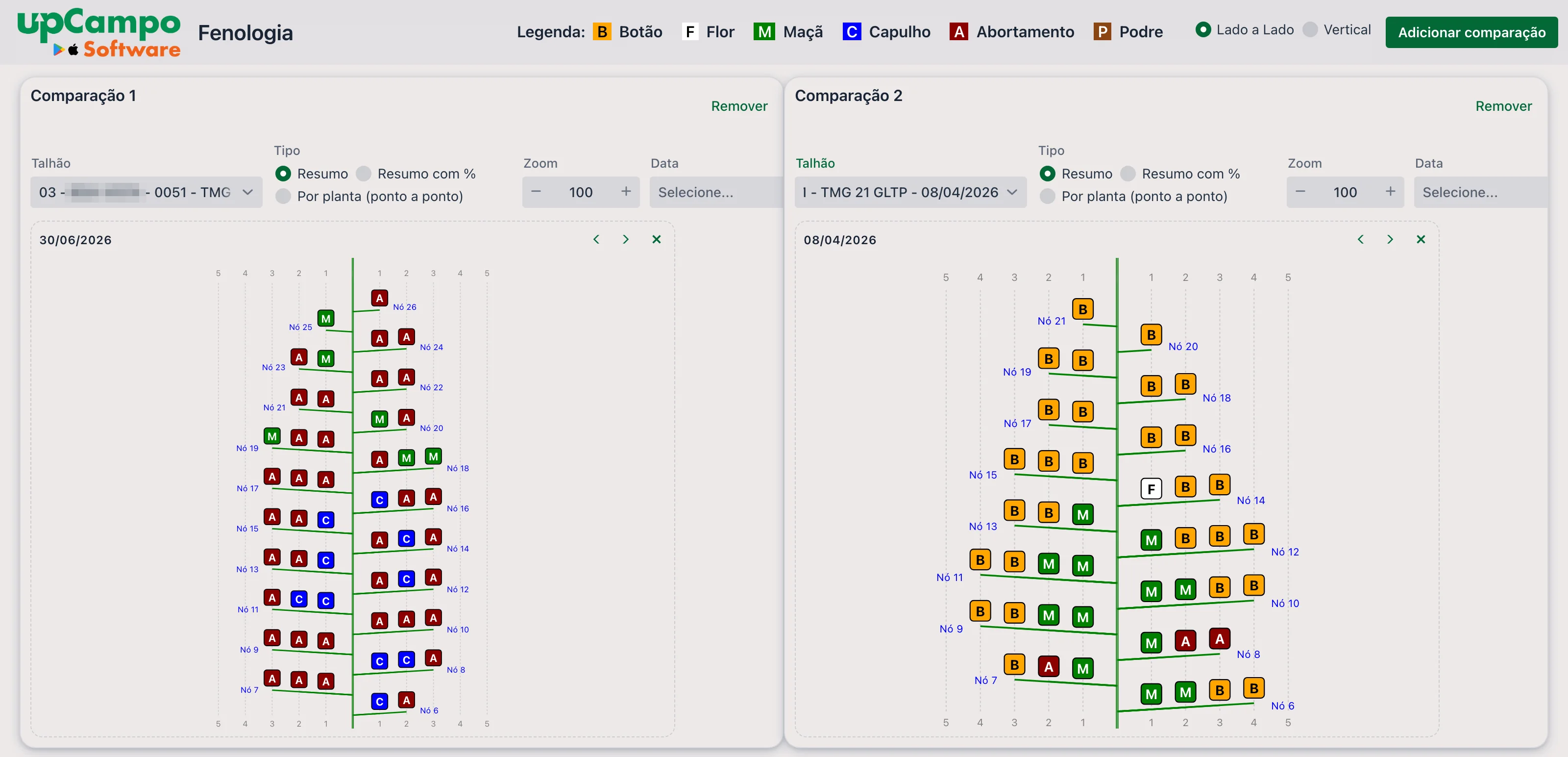
When the measurement shows up. The drawings are not built the moment the page opens: an upCampo routine prepares them every 7 minutes, from what has already synced. Counting the phone's sync, a plant measured in the field usually shows up within a few minutes. The dashboard reads the data when it opens — to see what came in afterwards, reload the page.
Height, and ideal height, on the dashboard
Web portal: upCampo > Scouting
The Scouting tab on the home screen shows each scouting in a column, with the field, crop, variety, days after planting and after emergence, stage and who measured — and, further down, the plant measurements.

Among the measurements are STAND, Height, Node Qty and a -- Ideal Height row: the height the crop should have on that day, according to the registered curve. In the example, the plant is at 96.28 cm and the ideal for that moment is 100 cm — in other words, practically as expected.

Value history, day by day
The value in the grid is a button. Clicking the height — or any other measurement in the column — opens the Value History window, with the whole season for that field in a single chart:
- the Height line, with what was measured at each scouting;
- the Ideal Veg. Growth line, which is the registered curve;
- the Work Order/Activity bars, marking the days when there was an application.
The bottom axis shows the date and DAE of each point. Below the chart, a table repeats the numbers and adds the Difference from previous, the Average per day and the Average per DAE — the growth between one scouting and the next. The Map tab, at the top, shows where the points were taken.
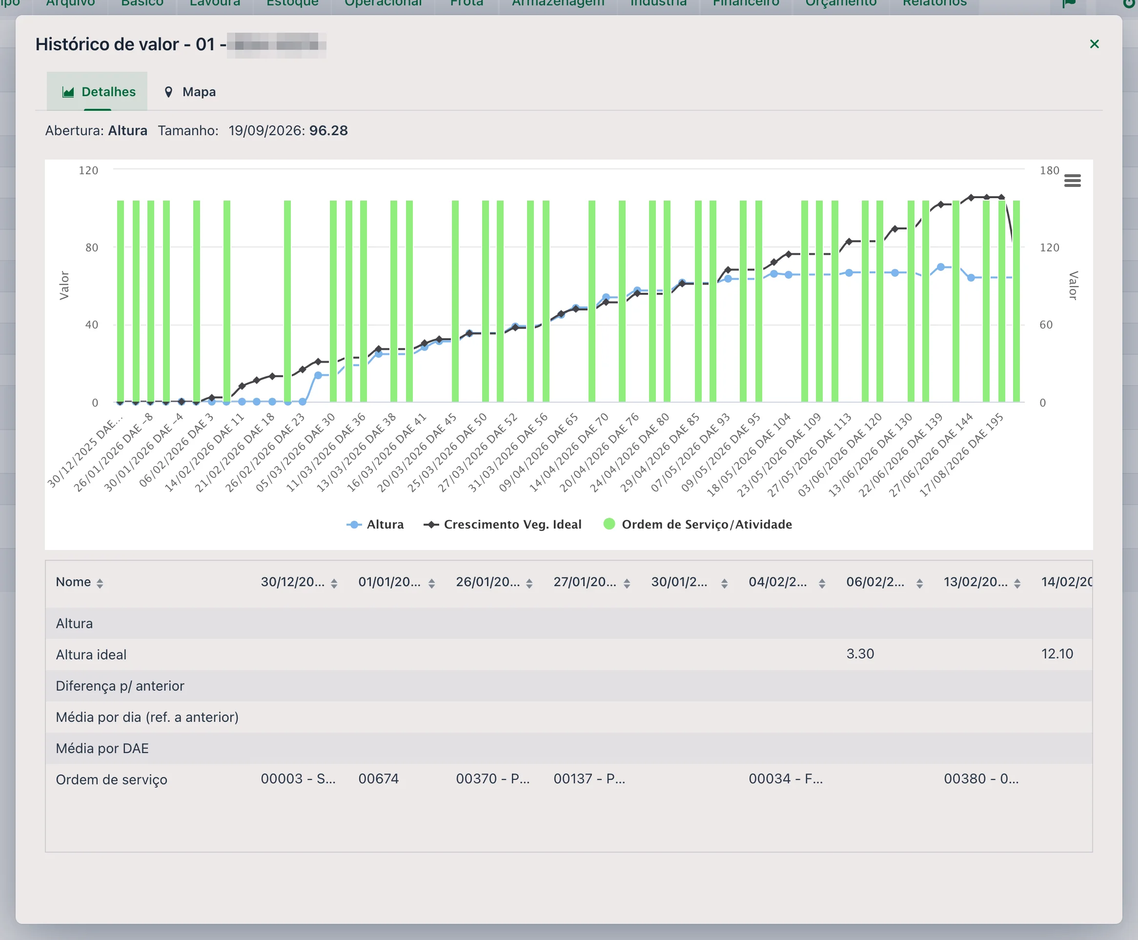
This is the reading that shows the pace: two equal measurements can mean different things depending on how the plant was growing before — and the work order bars help connect a change of pace to an application.
3. The reports
Web portal: Reports → Survey theme
The reports below ask for the same filters (MON.02.03 (formerly 001.O) also has Estimated weight): Date (period, required), Quadra(s) and Sector. Quadra is the old name for a field; left blank, all are included. They only consider the cotton phenology pest — the same one the dashboard uses. How to run and export reports is in the Quick Guide - Reports.
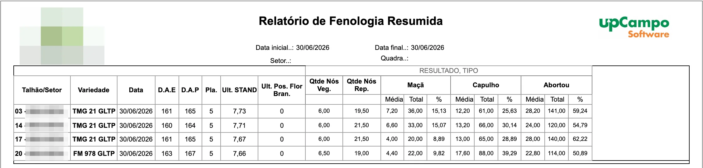
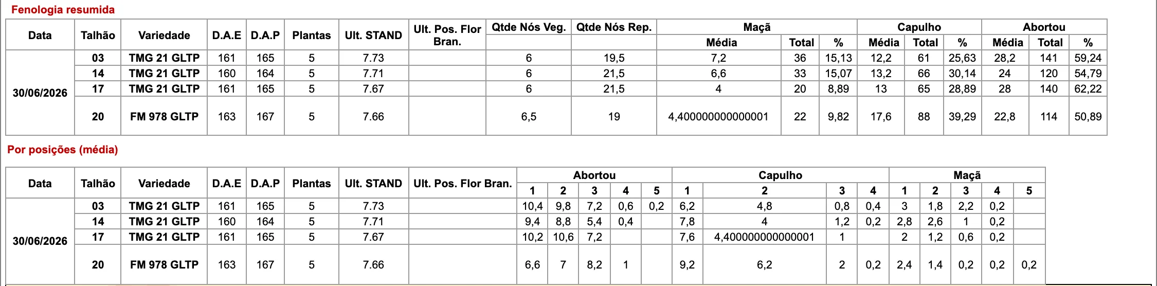
The field in numbers: one row per field and scouting date, with Variety, D.A.E and D.A.P (days after emergence and after planting, counted from Season Planting), Pla. (how many plants were assessed), Last STAND (the last stand recorded up to that date), Last White Flower Pos. and the averages of Veg. Node Qty and Rep. Node Qty. Then comes a block for each state found in the period — Square, Flower, Boll, Open boll and Aborted —, each with three columns:
- Average — how many structures of that state per plant;
- Total — how many were marked in the field;
- % — that state's share of all structures marked in the field on that day.
Each plant's sheet, grouped by field and by point (with the scout who measured): Height, Total Nodes, Veg. Nodes, Veg. Squares and Rep. Nodes, and the count of Square, Flower, Boll, Open boll, Aborted and the Total for that plant. At the end of each field, a Summary (average) of the measurements. It is for checking the collection plant by plant. To see the plant drawn node by node, use MON.02.02 (formerly 001.M2), just below.

The most complete report for node-by-node mapping, and the one that takes the dashboard's plant drawing to paper. It opens with two tables for the period:
- Summary phenology — the same numbers as MON.02.01 (formerly 001.N) (plants, Last STAND, nodes and, per state, Average, Total and %), field by field;
- By position (average) — for each state, how many structures per plant there are at each position on the branch, from 1 to 5. This is where you see, for example, that abortion is concentrated at positions 1 and 2 and barely reaches 4.
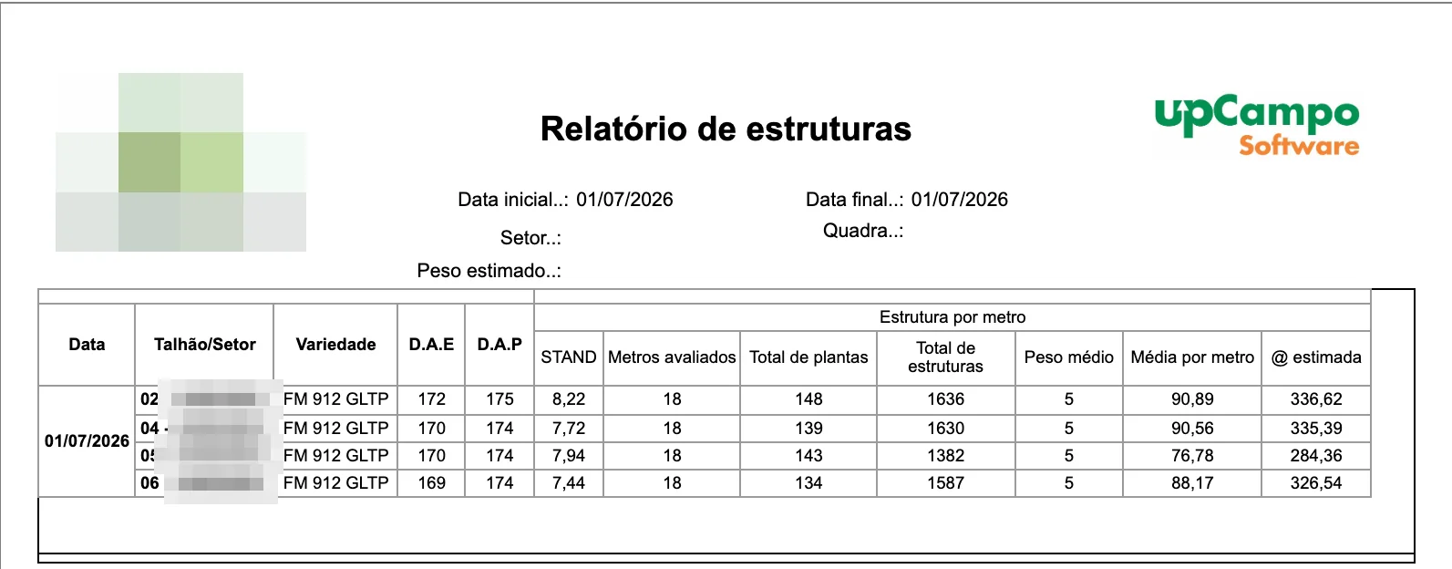
It doesn't use the node-by-node measurement: it reads the Structure per meter pest, entered in the same scouting in the app. The report shows, by field and date:
- STAND — total plants ÷ meters assessed;
- Average per meter — total structures ÷ meters assessed;
- Estimated @ — the estimated yield in arrobas per hectare, using the calculation below.
The 11,111 is the meters of row per hectare at 0.90 m row spacing, and that number is fixed in the calculation — for a field planted with a different spacing, the estimate has to be adjusted by hand. The 15 converts kilograms into arrobas. In the screenshot example, 90.89 structures per meter × 5 g ÷ 1,000 × 11,111 ÷ 15 gives 336.62 @/ha. The numbers are from a real field and are there to show the calculation, not as a yield benchmark.
Other cotton phenology reports under the same theme, for those who need a specific cut: MON.02.P05 (formerly 001.Qb) - Phenologies: Height, STAND, Node Qty, MON.02.P06 (formerly 001.R) - White Flower Position & Node Qty and MON.02.11 (formerly 001.H) - Phenology - Summary - Last of each WEEK.
- The farm sees where the plant is holding its load and where it is aborting, node by node, and not just how much there is per meter
- The field's development becomes visible by comparing dates side by side, from square to open boll
- Variation between plants shows up in Per plant, and an out-of-line measurement is caught before it becomes part of an average
- The numbers in MON.02.01 (formerly 001.N) and the sheets in MON.02.05 (formerly 001.M) are ready for season follow-up and for the records
❓ Frequently asked questions
I measured the plant in the app and it didn't show up on the dashboard. Why?
In upCampo, the phenology dashboard drawings are prepared every 7 minutes from what has already synced. Check that the phone synced, wait a few minutes and reload the page — the dashboard only reads the data when it opens. If it still doesn't show up, check that the measurement was made in the Detailed Cotton Phenology class, and not as a regular count.
What is the difference between Summary and Summary with % on the dashboard?
Summary shows, at each node and position, only the most frequent state among the plants measured. Summary with % shows all the states found at that position, each with its percentage. The first is the quick read; the second shows how divided the field is.
Does the position percentage count the plants where it was empty?
No. In upCampo, a position marked as absent in the app is not saved, so the dashboard percentage is out of the plants that had some structure at that position. A position that existed on only one plant can show 100%. To see how many plants it existed on, use the dashboard's Per plant type or the MON.02.02 (formerly 001.M2) - Detailed Phenology - Plant Map report.
Can I measure more than one plant at the same point?
The app allows it, but the phenology dashboard draws one plant per point, and the two plants would fall into the same drawing, overlapping. In upCampo, the node-by-node mapping routine is to open a new point for each plant measured.
Which report do I use to follow cotton phenology field by field?
MON.02.01 (formerly 001.N) - Summary Phenology: by field and date, it shows the percentage, total and average per plant of squares, flowers, bolls, open bolls and abortions, plus the last stand and the averages of vegetative and reproductive nodes. To see each plant drawn node by node, use MON.02.02 (formerly 001.M2) - Detailed Phenology - Plant Map.
How do I compare the same crop on two dates?
On the phenology dashboard, choose the field with the first date, tap Add comparison and choose the same field with the second date in Comparison 2. With Side by Side selected, the two drawings sit next to each other.
Can my farm use node-by-node phenological mapping?
It is a custom-built feature: it is currently configured for one specific customer's Cotton 2026 season. To use it on another farm, contact upCampo support — collection depends on how the cotton phenology pest is registered, and the dashboard is prepared for each farm and season.